Introduction
Before defining an electronic analogue computer, it is helpful to define the more general term analogue device. To make this easier, here is a list of analogue devices: clocks (sundials, water clocks, pendulum clocks, analogue watches), the astrolabe, slide rules, the governor of a steam engine, the planimeter (a simple device that measures the area of a closed shape), Kelvin's mechanical tide predictor, servomechanisms (thermostats, the cruise control of a car), the musical synthesizer, the light sensor in digital cameras (sic), an ordinary mercury thermometer, a bathroom scale, analogue-signal television, and the speedometer of a car.
A 16th century astrolabe, showing a tulip rete and rule
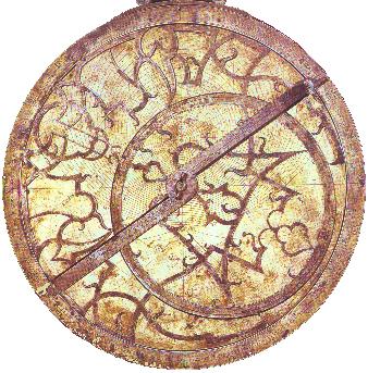
NB Astrolabes are mechanical devices used to locate and predict the positions of the Sun, Moon, planets and stars; determine local time given local longitude and vice-versa; surveying; and triangulation. The astrolabe was used during 200 BC to the 18th century, when it was replaced by the sextant.
The word "analogue" means "a similar thing" and in an analogue device the output is meant to model the actual quantity we are interested in. Thus a bathroom scale gives the analogy of the position of an arrow to the weight of a person.
An instrument with a read-out or dial that shows information using arrows, cursors, or levels, as opposed to displaying changing numerical digits, is usually an analogue device. By contrast, a digital device deals in digital quantities, which are specific numbers, such as 2 or 2.716. An analogue value requires an indefinite decimal expansion. If the digital value measures a physical quantity then it is only approximate. All measurable quantities, such as length, weight and speed are continuous in nature. Thus a piece of wood is never exactly a metre long, if only because its ends cannot be perfectly flat.
We are familiar with examples of analogue and digital versions of the same device. Thus a digital clock gives a numeric display (eg "14:37"), whereas an analogue clock has arms that move continuously. Digital storage of music on CDs decomposes sound into patterns of ones and zeroes, with no gradations in between. In contrast, a gramophone record (or cassette tape) represents sound as a continuous wave-form with smooth peaks and troughs. It is important to remember that it is the internal representation of data that makes a device analogue or digital, not the form in which the final result is presented. Thus an analogue device like a thermometer can have a digital read-out, and conversely, a digital device such as a PC can emit sound through the speakers (sound waves are analogue).
Analogue and digital devices represent numerical values in fundamentally different ways. An analogue device establishes a direct proportion between the quantity represented and the position of a sliding or rotating part in a mechanical system, or the voltage in an electrical circuit. This is the origin of the term “analogue”. The mechanism can take on any value in a given range. In a digital device each part can only take on the values 0 or 1, so that each component (usually a transistor) represents only a part of a number. Hence a group of devices is needed to represent a value. Contrast this with an analogue computer, where a single capacitor represents one continuous variable.
In general, an analogue device is an apparatus that processes continuous information in order to solve a problem, give a reading or to generate output from input. The measured analogue signal has an infinite number of possible values, which can be levels of voltage, resistance, rotation or pressure. By contrast, in a digital device, data is represented in a granular way, with no possible intervening values. The solar system is analogue in the sense that the planets can assume any particular position in space. In quantum physics, the atom is seen as digital in the sense that electron orbits can only have discrete sizes, with no intervening states being allowed.
The terms “analogue” and “digital” are somewhat deceptive, since the essential difference is between continuous and discrete internal representation, not between gauges and digital read-outs.
Just to make life complicated, there are instances where the digital-analogue distinction is blurry, eg a sound wave shown on a computer screen looks analogue, even though the monitor screen has a fixed number of dots, ie the display is digital.
Definition
A computer is a device that, once it has been suitably set up or programmed, can perform calculations independently of the operator. An analogue computer is a form of computer that uses continuous physical phenomena, such as electrical, mechanical, or hydraulic quantities, to model the problem being solved. An electronic analogue computer is an analogue computer that uses electronic components, such as valves or semi-conductors. A programmable analogue computer is one that manipulates data according to a list of instructions. Thus, if the instructions are changed the computer can solve a different problem.
Note that instructions should not be confused with data. The data fed into a computer are the numerical values on which it is to operate, whereas its instructions specify how it is to operate on the data.
An analogue computer does not "read" instructions in the way that a digital computer does. Instead of using an instruction file (ie a program), its instructions are contained in its setup, eg in the way it has been cabled together for the particular problem-solving task. Although nearly all computers are programmable, there are exceptions, eg special-purpose analogue computers have been made expressly to solve a single problem or to model a particular system.
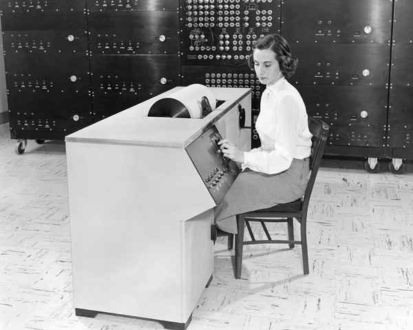
A differential analyser at the Lewis Flight Propulsion Laboratory, 1951 (photo: NASA)
The limited precision of analogue devices is counterbalanced by their simplicity and consequent economy of manufacture. In a digital device, an ensemble of parts is needed to represent a number. Essentially, a digital device can only perform addition. A sine is calculated by evaluating a power series, with the multiplications this implies carried out by a series of additions. Consequently, digital evaluation of a sine function is both complex and processor intensive, compared with an analogue device.
Unlike their analogue cousins, digital devices, such as a mechanical calculator or an electronic digital computer, are usually general-purpose tools that can be easily used for a wide range of computations. If a digital device can calculate a sine function, it can be re-programmed to calculate a logarithm or Bessel function. An analogue mechanism for the sine function, however, would be no use for a logarithm. Consequently, analogue devices are normally composed of independent parts, each designed to perform a single, distinct kind of calculation. Because the parts are independent they can all act simultaneously in parallel. Therefore, analogue devices are well suited to real-time applications, in which the calculation must keep step with events in the external world. In contrast, digital devices are sequential in nature, as they reuse a single calculating unit for each step of the calculation, and operate on data one step at a time. Hence the speed of execution slows down as the complexity of the calculation increases.
The history of computation began with digital calculating aids: the counting table and the abacus. Although simple to make, and not requiring sophisticated construction methods, they provided a useful degree of precision and were simple to use. Napier’s invention of logarithms reduced multiplication to the simpler operation of addition. This made possible the slide rule, a simple, yet very effective analogue device which offered limited but serviceable precision. Mechanical digital calculating devices first became widely available in the late nineteenth century, when improved manufacturing techniques made them economical. However, their slowness restricted them to addition in commercial environments.
The first half of the twentieth century saw much progress in the technology of mechanical analogue devices. A particular focus was the need to handle the real-time calculations required in military applications, such as targeting. During World War II, electronic technology advanced to make it possible for digital devices to perform higher mathematical functions, at speeds comparable to those of mechanical analogue devices. The same technology created improved analogue devices that competed effectively with digital ones in many areas until well through the 1960s. However, in the 1970s the remarkable cost reductions of electronic digital devices finally enabled them to supplant analogue devices as the dominant technology for calculation.
Currently, digital computing rules the day and little research is being done in analogue computing, in sharp contrast to the massive resources being lavished on digital technology. However, it would take a brave person to predict that analogue computers will never again become important in the future. Writing in 1969, KN Dodd opined, "For example, a slide rule is an entirely different entity from a modern digital computer. They have their own separate uses and there is no question of the one ever replacing the other." The slide rule was made entirely obsolete by the electronic calculator about six years later.
Postscript in 2016: Quantum computers, which are analogue devices, are in their infancy, but they have the potential to become far more powerful than digital computers.
Uses
Among other uses, computers can analyse something or control a device. The physical system to be analysed may be a pendulum, an atom, a nuclear reaction, the weather, the economy, or the solar system. To analyse means to study the behaviour of such a system. Analogue computers perform arithmetical calculations, as well as integration, differentiation and the evaluation of trigonometric and other functions. A differential analyser is an analogue computer that solves differential equations. A computer-controlled device performs a given function, eg an automatic pilot machine, a washing machine, a pocket calculator or a mobile phone.
During World War II, mechanical analogue computers were used to control guns. An analogue computer would receive the firing ship's location, heading, and speed, plus the wind direction, and other parameters, as well as operator-entered data concerning the type of projectile, the amount of explosive charge and, most importantly, the location of the target. The analogue computer would then control the aiming of the gun. From 1950 to 1965, electronic analogue vacuum-tube computers were used to design, test and run civilian and military equipment, like aircraft, ships or rockets. Analogue computers have been widely used in simulations of aircraft, nuclear-power plants, and industrial chemical processes. Other major uses included analysis of hydraulic networks (eg the flow of liquids through a sewer system) and electronics networks (eg the performance of long-distance circuits).
One of the more common modern applications of analogue devices is in process control. A simple analogue circuit using a few operational amplifiers may be used to control the temperature of an industrial process where the use of a digital computer is not warranted. Stand-alone analogue computers are no longer used.
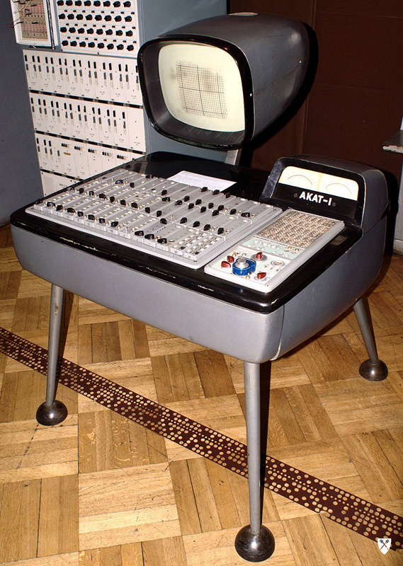
Polish analogue computer AKAT-1 (photo: Topory)
In an analogue computer, physical quantities such as voltages and shaft rotations are made to obey mathematical relations analogous to those of the original problem. The analogy is valid when the equations describing the operation of the computer system are mathematically identical to those describing the real problem.
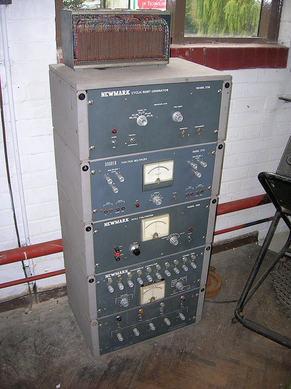
A large electronic analogue computer, such as that shown earlier, might comprise 200 operational amplifiers, twenty servomechanisms for performing multiplication etc, one or two electrically operated plotting tables, and 100 manually adjustable potentiometers. A patch panel (or plugboard), similar to a manual telephone switchboard, is needed to connect all these components together, in order to model a particular problem. The patch panel has thousands of sockets connected to the inputs and outputs of the amplifiers, servomechanisms, and potentiometers. These sockets can be interconnected as required by plugs and wires. Since making these connections is time-consuming, the patch panel can be detached from the computer, so that the connections can be made at leisure, allowing others to use the computer. The patch panel is then inserted in a single operation. In effect, the patch panel acts as a set of stored instructions. Output is shown on a voltmeter, oscilloscope or pen plotter.
Analogue computers represent constants and variables with proportional analogue voltage levels. These are then processed by various electronic circuits that perform the mathematical operations in analogue form. The key processing circuit is the operational amplifier, a device whose output current is proportional to its input potential difference. It can be easily reconfigured to perform a wide range of mathematical operations, such as addition, subtraction, multiplication and division by a constant, integration and differentiation. The operational amplifier can even be configured to do logarithmic and trigonometric operations with special non-linear feedback circuits. The amplifiers are placed in what is called a "feedback" circuit, where some of the output signal is fed back to the input. The nature of the feedback circuit determines the mathematical operation performed by the amplifier.
The operational amplifier may be a valve or a semi-conductor. A high-gain amplifier is also called a DC amplifier. A simple amplifier is one that has two inputs, e1 and e2, and one output, e3. The inputs e1 and e2 are voltages, while the output, e3, is the difference between these two, and is also a voltage. Such an amplifier responds only to the differences of its input. If the output is scaled by a factor, A, then this is called the gain of the amplifier. Most amplifiers closely approach the ideal of infinite input resistance (no current flowing in) and zero output resistance (high current output).
A signal is an electrical current or potential which conveys information in an analogue computer. For example, in sound recording, fluctuations in air pressure (ie sound) strike the diaphragm of a microphone, which causes corresponding fluctuations in a voltage or the current in an electric circuit. The voltage or the current is said to be an "analogue" of the sound.
Another basic component used in analogue computers is the potentiometer. It is a resistance with a sliding tap. It is used to multiply by a constant, which is set on a dial. The volume control on an audio amplifier is a potentiometer.
Programming
Programming an analogue computer involves writing out the equations to be solved, converting them to a block diagram, then wiring the various computing elements together with pluggable cords on a large patch panel. One goes through a procedure of general analysis, data preparation, analogue circuit development, and patch panel programming. It may be necessary to do test runs of subprograms to examine partial-system responses, before eventually running the full program to derive specific and final answers. Normally, eight major steps are involved:
1. If possible, the problem is described using a set of mathematical equations. Alternatively, the system configuration and the interrelations of component influences are defined in block-diagram form. Each block is described in terms of black-box input-output relationships.
2. It may be necessary to rearrange the description of the system (equations or system block diagram) in a form that suits the capabilities of the computer. This is to avoid duplications or excessive numbers of computational units, and to avoid recursive formulas.
3. An analogue circuit diagram is sketched out using the assembled information. The diagram shows in detail how to program the computer to handle the problem.
4. Since it is necessary to operate within the operational ranges of the computer, system variables and parameters may need to be scaled. As a result, the analogue circuit diagram may need revision.
5. The computer patch panel is wired according to the circuit arrangement.
6. The initial conditions of the system model are established and numerical values are set up on the attenuators (devices that reduce signal amplitude). Test values are checked.
7. Initial answers are generated by running the computer, giving the “feel” for the system.
8. To check the responses for specific sets of parameters and to explore the influences of problem changes, it is necessary to run the computer multiple times.
Limitations
The drawback of the mechanical-electrical analogy is that electronics are limited by the range over which the variables may vary. This is called dynamic range, much like dynamic range in photography. An electronic analogue signal is composed of four basic components: DC and AC magnitudes, frequency, and phase. The real limits of range of these characteristics constrain analogue computers. Some of these limits include noise, non-linearities, temperature coefficient (the relative change of a physical property when the temperature is changed by a degree), parasitic effects within semiconductor devices, and the fixed charge of an electron.
All mechanical and electrical devices are subject to disturbing influences, called "noise". If a digital device suffers a small disturbance, no error will arise in its indication. This is due to the granularity of its values, ie 1 does not become 0, nor vice versa with small disturbances. Binary representation is verbose, but the benefit is robustness. No analogue device is immune to noise. If its state is accidentally disturbed, the new state represents a valid value of the variable. Hence the precision of an analogue computer depends on keeping the noise low. High precision, whether in the machining of mechanical parts, the manufacture of electronic components, or the isolation of a circuit from external electromagnetic influences, is always difficult and expensive to obtain.
Any calculation that can be performed by an analogue computer can be performed more accurately by a digital computer. However, until the 1960s, analogue computers were cheaper and faster.
A 1960 Newmark analogue computer, made up of five units. It was used to solve differential equations